German Tank Problem

November 27, 2025

Introduction #

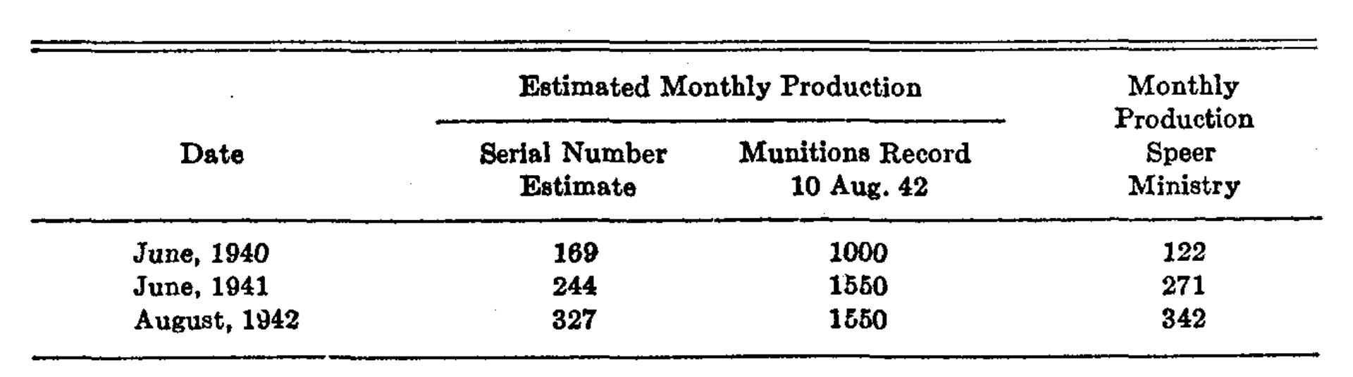
In this article, we review the famous German Tank Problem which refers to the estimation of the number of German tanks in production on a monthly basis by the Allied forces based on observations of the serial numbers of tanks, either through capture or espionage. The original report discussing the details of this problem was performed by Ruggles and Brodie, see [1] , and Figure 1 for an extract of a table (pg. 89) from the report depicting estimates for tank production both via statistical and intelligence means. Additionally, a proof of the estimators suggested to in the Ruggles and Brodie report was performed by Goodman, see [2] .

Problem Statement #

In mathematical terms, assume that we have an unknown number $N$ of German tanks being produced on a monthly basis, and that each tank is identified by a unique serial number. Assume further that the serial numbers can be mapped to the natural numbers (starting at one) whilst preserving order, where the order can be interpreted by the order in which they are produced. Assume further that we have observed $k$ tanks and our aim now is to determine an estimator, $\hat{N}$, for $N$ which is unknown.

Estimation #

Let $X_{1}, \ldots, X_{k}$ denote the random variables corresponding to the serial markings observed on German tanks. We assume that each $X_{i}$ is sampled uniformly from $\lbrace 1, \ldots, N \rbrace$ without replacement. In particular, we have that for any $i \in \lbrace 1, \ldots, k \rbrace$

Something to note is that, while the observations are identically distributed, they are not independent since we assume no replacement (i.e. serial numbers are not reused).

For the purpose of calculations below, as the order of the statistics is not relevant (we do not care in which order the serial numbers were obtained), we consider the order statistics $X_{(1)} < \cdots < X_{(k)}$, which have a joint density

Now, there are numerous estimators that one could use for $N$, but one must be wary of if they are biased and be conscious of their variance.

Maximum Observed Value #

If the tank number is $50$, then we know that $N \geqslant 50$, therefore a naïve first estimate could be the maximum observed value.

Let $M := \max \lbrace X_{1}, \ldots, X_{k} \rbrace = X_{(k)}$ denote the random variable corresponding to the maximum observed value, and $\hat{N}_{\text{max}} = M$ the estimator for $N$.

We now wish to determine whether $\hat{N}_{\max}$ estimator is biased and what its variance could be, for which we need the density of $M$. Whilst it is true that $X_{k}$ is uniformly distributed, $X_{(k)}$ is the ordered statistic, and is heavily biased towards larger values, and therefore is not uniformly distributed - therefore, we need to derive the density of $M$.

Let $m \in \lbrace 1, \ldots, N \rbrace$, then the total number of possible outcomes of our samplings is $\binom{N}{k}$, and out of these, the total number of outcomes where the maximum is $m$ is the number of ways of choosing $k - 1$ numbers below $m$, i.e. $\binom{m - 1}{k - 1}$. Therefore

Hence

and

In particular, we see that

i.e. that the estimator is biased, and will systematically underestimate $N$, with the underestimation gap becoming more severe with increasing $N$.

Method of Moments #

We know that each $X_{i}$ is uniformly distributed across $\lbrace 1, \ldots, N \rbrace$, and with that, for all $i \in \lbrace 1, \ldots, k \rbrace$

giving us the identity $N = 2 \mu - 1$. If we are able to obtain an estimator for $\mu$, we can also do so for $N$. Letting $\bar{X} := \frac{1}{k} (X_{1} + \cdots + X_{k})$ denote the sample mean, $\bar{X}$ provides an unbiased estimator of $\mu$, i.e.

and indeed, with that, we are able to obtain the estimator $\hat{N}_{\text{MoM}} := 2 \bar{X} - 1$, for which we have

Maximum Likelihood #

Denote by $\boldsymbol{x} = (x_{1}, \ldots, x_{k})$ an observed sample of serial numbers, and $\boldsymbol{X}= (X_{1}, \ldots, X_{k})$. Then for $N \in \lbrace k, k + 1, \ldots \rbrace$, the likelihood function (representing the probability of observing this specific sample given a population size $N$) is defined as

For brevity, in the following we write $L (N)$ to denote $L (N| \boldsymbol{x})$. Now, we want to determine the maximum likelihood - the likelihood is strictly decreasing (since its reciprocal is strictly increasing) in $N$,

i.e. $L (N + 1) < L (N)$ for any $N \geqslant \max \lbrace x_{1}, \ldots, x_{k} \rbrace$. Therefore, the $N$ which maximises the likelihood is $\max \lbrace x_{1}, \ldots, x_{k} \rbrace$, giving the estimator

which we have covered above.

“Best” Estimators #

A question one can ask themselves is, what is the best estimator to $N$? Well, this entirely depends on what is mean’t by best. One common technique that is used in literature is finding estimators that minimise the mean squared error (MSE), although other loss functions can also be used, see Chapter 7.3.4 of [3] for a discussion on the use of alternative loss functions.

Definition: The mean squared error of an estimator $W$ of a parameter $\theta$ is

where $\text{Bias}_{\theta} (W) := \mathbb{E}_{\theta} (W) - \theta$.

Having defined the MSE, we can now search for an estimator that has the best MSE across all parameters $\theta$. But this is not always possible, in fact, one can often find two estimators that outperform each other with respect to the MSE across different parameter ranges. The reason for this difficulty is that the space of all estimators is quite large.

UMVUE #

To obtain a recommended estimator, many resort to restricting to the space of unbiased estimators, i.e. those such that $\mathbb{E}_{\theta} (W) = \theta$. In such a scenario, the MSE simply corresponds to the variance of the estimators, and therefore the estimators we seek are those that have uniformly smallest variance.

Should I always use an unbiased estimator? No. In many cases, one can make a large improvement on the variance by forgiving some unbiasedness, and with that achieve a much better MSE. Although unbiased estimators as ideal, they are not always the best!

Definition: (UMVUE) An estimator $W^{\ast}$ is the uniform minimum variance unbiased estimator (UMVUE) of $\theta$ if it satisfies $\mathbb{E}_{\theta} (W^{\ast}) = \theta$ for all $\theta$, and for any other estimator $W$ with $\mathbb{E}_{\theta} (W) = \theta$, we have $\mathbb{V}_{\theta} (W^{\ast}) \leqslant \mathbb{V}_{\theta} (W)$ for all $\theta$.

Finding the UMVUE is not an easy task, it may not exist, and even if it does, it is difficult to know from first principles how to obtain one. It could be possible that from the estimators already obtained for a given problem, that at one of them is the UMVUE, but how can one know unless the inequality can be proven across all possible estimators.

Cramér-Rao Inequality - A Short Detour #

One way to get around the issue of knowing when to stop is to know first what is the lowest possible variance one could possible strive to obtain, and then check if your estimator attains this bound – this is where the Cramér-Rao inequality comes in.

Theorem: (Cramér-Rao Inequality) Let $X_{1}, \ldots, X_{n}$ be a sample with pdf $f (\boldsymbol{x} | \theta)$, sample space $\mathcal{X}$, and parameter $\theta$, and let $W (\boldsymbol{X}) = W (X_{1}, \ldots, X_{n})$ be any estimator satisfying

or equivalent for discrete random variables. Then

where $\mathbb{I}_{\theta}$ is called the information number, or Fischer information of the sample, and is defined as

Corollary: (Cramér-Rao Inequality - Unbiased Case) Let $X_{1}, \ldots, X_{n}$ be a sample with pdf $f (\boldsymbol{x} | \theta)$ and let $W (\boldsymbol{X}) = W (X_{1}, \ldots, X_{n})$ be an unbiased estimator with $\mathbb{V}_{\theta} (W (\boldsymbol{X})) < \infty$. Then

The Cramér-Rao inequality is quite remarkable and also quite intuitive - it tells us that as more information is made available (i.e. as $\mathbb{I}_{\theta}$ increases), we can, in theory, obtain estimators that have smaller and smaller variances. Although, the attainment is not guaranteed.

If we have found an estimators that attains this bound, then we know (assuming that the conditions are met) that our estimator is optimal with respect to the variance, and is a UMVUE if it is also unbiased. Thankfully, the requirements for attainment of the Cramér-Rao bound are simple, although again, these requirements do not provide a means of constructing the optimal estimator.

Corollary: (Attainment) Let $X_{1}, \ldots, X_{n}$ be a sample with pdf $f (\boldsymbol{x} | \theta)$ and let $W (\boldsymbol{X}) = W (X_{1}, \ldots, X_{n})$ be any estimator satisfying the Cramér-Rao conditions. Then $W (\boldsymbol{X})$ attains the Cramér-Rao lower bound if and only if there exists a function $a (\theta)$ such that

We should note that the key assumption of the Cramér-Rao theorem is the requirement that we can differentiate under the integral sign, a condition that needs to be checked and is not always true.

Can we obtain a Cramér-Rao bound for our German tank problem? Unfortunately, no. For the German tank problem, we have

in particular, the support of our density depends on our parameter $N$. Due to this, we cannot simply differentiate under the integral without taking into consideration the boundary terms of the support. Let $S_{N} := \lbrace \boldsymbol{x} = \lbrace x_{1}, \ldots, x_{k} \rbrace | \max (\boldsymbol{x}) \leqslant N \rbrace$ denote the support of $f$, then, by the Leibniz rule for differentiating an integral (apply counting measure and proceed usually), for any estimator $W$ of $N$

where the Boundary Terms come from the dependence of the support on the parameter $N$, and are non-zero. As such, the Cramér-Rao bounds do not apply.

Constructing the UMVUE #

Thankfully, there exists some developed theory for constructing better unbiased estimators (those with lower variance), and also the UMVUE. Before we state these results, we need to understand what is a sufficient statistic.

A sufficient statistic for a parameter $\theta$ is a statistic that, in a certain sense, captures all the information about $\theta$ contained in the sample, i.e. if $T (\boldsymbol{X})$ is a sufficient statistic for $\theta$, then any inference about $\theta$ should depend on the sample $\boldsymbol{X}$ only through the value of $T (\boldsymbol{X})$.

Definition: (Sufficient Statistic) A statistic $T (\boldsymbol{X})$ is a sufficient statistic for $\theta$ if the conditional distribution of the sample $\boldsymbol{X}$ given the value of $T (\boldsymbol{X})$ does not depend on $\theta$.

How can we know if we have a sufficient statistic? For this, there is a simple result called the Factorisation Theorem, see [3] (Theorem 6.2.6), that allows to us to quickly identify such statistics.

Theorem: (Factorisation Theorem) Let $f (\boldsymbol{x} | \theta)$ denote the joint pdf of a sample $\boldsymbol{X}$. A statistic $T (\boldsymbol{X})$ is a sufficient statistic for $\theta$ if and only if there exists functions $g (t| \theta)$ and $h (\boldsymbol{x})$ such that, for all sample points $\boldsymbol{x}$ and all parameters $\theta$

Through the concept of sufficiency, we arrive at the remarkable result by Rao-Blackwell, see [3] (Theorem 7.3.17), which allows us to improve upon any unbiased estimator if one has access to any sufficient statistic for $\theta$, no matter how crude. This process of applying the Rao-Blackwell theorem is called Rao-Blackwellisation.

Theorem: (Rao-Blackwell) Let $W$ be any unbiased estimator of $\theta$, and $T$ be a sufficient statistic for $\theta$. Define by $\phi (T) := \mathbb{E} (W|T)$. Then $\mathbb{E}_{\theta} (\phi (T)) = \theta$ and $\mathbb{V}_{\theta} (\phi (T)) \leqslant \mathbb{V}_{\theta} (W)$ for all $\theta$, that is $\phi (T)$ is a uniformly better unbiased estimator of $\theta$ (note, $\phi$ is not necessarily the UMVUE).

How about if I wanted to construct the UMVUE, and not just improve upon my estimator? For that, we rely on the concept of completeness and the Lehmann-Scheffé theorem, see [3] (Theorem 7.3.19, Theorem 7.3.23, Theorem 7.5.1) which also tells us that any UMVUE is unique!

Definition: (Completeness) Let $f (t| \theta)$ be a family of densities for a statistic $T (\boldsymbol{X})$. The family of probability distributions is called complete if $\mathbb{E}_{\theta} (g (T)) = 0$ for all $\theta$ implies $\mathbb{P}_{\theta} (g (T) = 0) = 1$ for all $\theta$. Equivalently, $T (\boldsymbol{X})$ is called a complete statistic.

Theorem: (Lehmann-Scheffé) Let $T$ be a complete sufficient statistic for a parameter $\theta$, and let $\phi (T)$ be any estimator based only on $T$ such that $\mathbb{E} (\phi (T)) = \theta$. Then $\phi (T)$ is the unique UMVUE of $\theta$.

That is, if we are able to find a complete sufficient statistic of our parameter $\theta$, then by conditioning any estimator on this statistic will necessarily yield the UMVUE.

Back to the German Tank Problem #

Having determined how to obtain the UMVUE, we now move to construct it for the German tank problem. Recall the estimators that we determined for $N$, in particular $\hat{N}_{\operatorname{MoM}}$ and $\hat{N}_{\max}$,

and

The first question we ask is, can we improve either of these via conditioning, i.e. via Rao-Blackwellisation? We can if at least one of our estimators is sufficient.

We start with checking $\hat{N}_{\operatorname{MoM}}$. Recalling the Factorisation Theorem, to show that an estimator is sufficient, it suffices to determine if we can factorise the density $f (\boldsymbol{x} |N)$ into

for some $h, g$. Knowing that

we see that it is not possible to write the indicator $\boldsymbol{1}_{\lbrace \max \lbrace x_{1}, \ldots, x_{k} \rbrace \leqslant N \rbrace}$ solely in terms of $\bar{X}$, and therefore also not solely in terms of $\hat{N}_{\operatorname{MoM}}$, therefore $\hat{N}_{\operatorname{MoM}}$ is not sufficient.

Although, looking at the density, we see that the estimator $\hat{N}_{\max}$ is sufficient, as one can write

and choosing $h \equiv 1$ and $g (\boldsymbol{x}, \hat{N}_{\max}) = \frac{1}{\binom{N}{k}} \boldsymbol{1}_{\lbrace \hat{N}_{\max} (\boldsymbol{x}) \leqslant N \rbrace}$ gives us the required factorisation.

So what does this all mean? Although $\hat{N}_{\operatorname{MoM}}$ is not a sufficient statistic, it is unbiased (unlike $\hat{N}_{\max}$), so we can condition it with the sufficient statistic $\hat{N}_{\max}$ to obtain a uniformly better unbiased estimate than $\hat{N}_{\operatorname{MoM}}$.

For brevity, let $M = \hat{N}_{\max}$ and define $\phi (m) := \mathbb{E} (\hat{N}_{\operatorname{MoM}} |M = m)$ for some $m \in \lbrace k, k + 1, \ldots \rbrace$. Then, as an estimator, $\phi$ can be written as

By the law of total expectation,

which allows us to write the estimator $\phi (M)$ as

In particular, by the Rao-Blackwell theorem, we have obtained the estimator $\hat{N}_{\operatorname{RB}} := \phi (M) = M \left( \frac{k + 1}{k} \right) - 1$ which provides a uniformly better unbiased estimator than $\hat{N}_{\operatorname{MoM}}$.

Indeed, we can see that

i.e. $\mathbb{V} (\hat{N}_{\operatorname{RB}}) <\mathbb{V} (\hat{N}_{\operatorname{MoM}})$ for $k > 1$.

Now, the question then is, is $\hat{N}_{\operatorname{RB}}$ the UMVUE? For this, we need to check whether the family of densities for the estimator $M = \hat{N}_{\max}$ is complete.

Let $g$ be any function of $M$ such that $\mathbb{E} (g (M)) = 0$, then it suffices to show that $\mathbb{P} (g (M) = 0) = 1$ for all $N$. Applying the definition of the expectation, we see that, under $k$ samples

Since $\binom{N}{k} > 0$, we can multiply out to obtain

We now show that $g (m) = 0$ for $m \in \lbrace k, \ldots, N \rbrace$ via an inductive argument. As a base case, consider $N = k$. Then

and therefore $g (k) = 0$. Assume now that the statement holds true for an arbitrary $N$, then we wish to prove this for $N + 1$. Indeed,

Since the case is assumed to hold true for $N$, we have that

and therefore

and hence $g (N + 1) = 0$, i.e. the case holds true also for $N + 1$, which concludes the inductive proof, i.e. $g (M) = 0$. In particular, we have

i.e. $M$ is also a complete statistic. In particular, that $\hat{N}_{\operatorname{RB}} := \phi (\hat{N}_{\max}) = M \left( \frac{k + 1}{k} \right) - 1$ is the UMVUE.

References

- Richard Ruggles and Henry Brodie (1947). An Empirical Approach to Economic Intelligence in World War II. 42 (237) : 72–91. doi:10.1080/01621459.1947.10501915 link
- Leo A. Goodman (1952). Serial Number Analysis. 47 (260) : 622–634. doi:10.1080/01621459.1952.10483442 link
- George Casella and Roger L. Berger (2002). Statistical Inference.